The Hough transform is a method for detecting parameterized objects, typically used for lines and circles in 2D space. Nowadays, with the proliferation of acquisitive devices, deriving a massive point cloud is an easy task. As we can also parameterize objects in 3D, Hough transform can be applied to detect planes in 3D point clouds as well.

Parameterization of a Plane

Similar to a line in 2D space, a plane in 3D can be described using a slope–intercept equation, where $k_x$ is the slope in x-direction, $k_y$ is the slope in y-direction, and $b$ is the intercept on z-axis:$$\begin{equation}z=k_xx+k_yy+b.\tag{1}\label{eq:1}\end{equation}$$With $\eqref{eq:1}$ we can simply parameterize a plane as $(k_x,k_y,b)$.

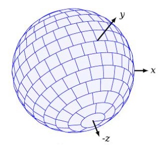
However, values of $k_x$, $k_y$, and $b$ are unbounded, which would pose a problem when we try to parameterize a vertical plane. Thus, for computational reasons, we can write the plane equation in the Hesse normal form, where $\theta$ is the angle between the normal vector of this plane and the x-axis, $\phi$ is the angle between the normal vector and z-axis, and $\rho$ is the distance from the plane to the origin:$$\begin{equation}x\cos\theta\sin\phi+y\sin\phi\sin\theta+z\cos\phi=\rho.\tag{2}\label{eq:2}\end{equation}$$As shown in Figure 1, the plane can be parameterized as $(\theta,\phi,\rho)$.

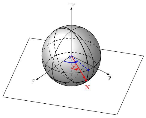
To find planes in a 3D point cloud, we have to calculate the Hough transform for each point, which is to say that we parameterize every possible plane that goes through every point in the $(\theta,\phi,\rho)$ Hough space. For instance, Figure 2 shows the parameterization of three points $(0,0,1)$, $(0,1,0)$, and $(1,0,0)$. Each point is marked as a 3D sinusoid curve in Hough space and the intersection which is marked in black denotes the plane defined by the three points.

Hough Methods

Basically, the algorithm for Hough transform can be described as a voting method, where we discretize the Hough space with a bunch of $(\theta,\phi,\rho)$ cells. A data structure called accumulator then is needed to store all these cells with a scoring parameter for every cell. Incrementing a cell means increasing the score of it by +1. Each point votes for all cells of $(\theta,\phi,\rho)$ that define a plane on which it may lie.

Standard Hough Transform

A most basic and naïve Hough transform algorithm for plane detection is outlined as follows:

Begin

Step 1: Traverse all the points in the point cloud $P$;

Step 2: For each point $\mathbf{p}_i$ in $P$, vote for all the $A(\theta,\phi,\rho)$ cells in the accumulator $A$ defined by this point;

Step 3: After the whole iteration, search for the most prominent cells in the accumulator $A$, that define the detected planes in $P$.

End

The standard Hough transform is performed in two stages: incrementing the cells, which needs $O(|P|\cdot N_\phi\cdot N_\theta)$ operations, and searching for the most prominent cells, which takes $O(N_\rho\cdot N_\phi\cdot N_\theta)$ time, where $|P|$ is the size of the point cloud, $N_\phi$ is the number of cells in direction of $\phi$, $N_\theta$ in direction of $\theta$, and $N_\rho$ in direction of $\rho$.

Probabilistic Hough Transform

In the standard Hough transform, the size of the point cloud $|P|$ is usually much larger than the number $N_\rho \cdot N_\phi \cdot N_\theta$ of cells in the accumulator array. We can simply reduce the number of points to improve the computational expense. Thus, the standard Hough transform can be adapted to the probabilistic Hough transform, which is shown as follows:

Begin

Step 1: Determine the size value $m$ and the threshold value $t$;

Step 2: randomly select $m$ points to create $P^m\subset P$;

Step 3: Do the standard Hough transform on the point set $P^m$;

Step 4: Delete the cells from the accumulator $A$ with a value that does not reach $t$, and search for the most prominent cells in $A$, that define the detected planes in $P$.

End

The $m$ points (with $m<|P|$) are randomly selected from the point cloud $P$, so the dominant part of the runtime is proportional to $O(m\cdot N_\phi\cdot N_\theta)$. However, the optimal choice of $m$ and the threshold $t$ depends on the actual problem, e.g., the number of planes, or the noise in the point cloud.

Adaptive Probabilistic Hough Transform

In order to find the optimal subsample of the point cloud, we can use an adaptive method to determine the reasonable number of selected points. The adaptive probabilistic Hough transform monitors the accumulator. The structure of the accumulator changes dynamically during the voting phase. As soon as stable structures emerge and turn into significant peaks, voting is terminated.

Begin

Step 1: Check the stability order $m_k$ of the list of $k$ peaks $S_k$ in the accumulator, if it reaches the threshold value $t_k$ then finish;

Step 2: Randomly select a small subset $P^m\subset P$;

Step 3: Do the standard Hough transform on the point set $P^m$;

Step 4: Merge the active list of peaks $S_k$ with the previous one, determine the stability order $m_k$, goto Step 1;

End

In this algorithm, The stability is described by a set $S_k$ of $k$ peaks in the list, if the set contains all largest peaks before and after one update phase. The number $m_k$ of consecutive lists in which $S_k$ is stable is called the stability order of $S_k$.

Progressive Probabilistic Hough Transform

The progressive probabilistic Hough transform calculates stopping time for random selection of points. The algorithm stops whenever a cell count exceeds a threshold.

Begin

Step 1: Check the input point cloud $P$, if it is empty then finish;

Step 2: Update the accumulator with a single point $\mathbf{p}_i$ randomly selected from $P$;

Step 3: Remove $\mathbf{p}_i$ from $P$ and add it to $P_\text{voted}$;

Step 4: Check if the highest peak in the accumulator that was modified by the new point is higher than the threshold $t$, if not then goto Step 1;

Step 5: Select all points from $P$ and $P_\text{voted}$ that are close to the plane defined by the highest peak and add them to $P_\text{plane}$;

Step 6: Search for the largest connected region $P_\text{region}$ in $P_\text{plane}$ and remove from $P$ all points in $P_\text{region}$;

Step 7: Reset the accumulator by unvoting all the points in $P_\text{region}$;

Step 8: If the area covered by $P_\text{region}$ is larger than a threshold, add it to the output list, goto Step 1;

End

In this algorithm, $P_\text{voted}$ is the point set of all the voted points before a plane is detected, $P_\text{plane}$ is the set of points in the detected planes, and $P_\text{region}$ denotes the largest connected region in $P_\text{plane}$. For determining the stopping time, the threshold $t$ is predicated on the percentage of votes for one cell from all points that have voted.

Randomized Hough Transform

As we know the fact that a plane is defined by three points. For detecting planes, three points from the input space are mapped onto one point in the Hough space. When a plane is represented by a large number of points, it is more likely that three points from this plane are randomly selected. Eventually, the cells corresponding to actual planes receive more votes and are distinguishable from the other cells. Inspired by this idea, we can come up with an algorithm described as follows:

Begin

Step 1: Check the input point cloud $P$, if it is empty then finish;

Step 2: Randomly pick three points $\mathbf{p}_1$, $\mathbf{p}_2$, and $\mathbf{p}_3$ from $P$;

Step 3: If $\mathbf{p}_1$, $\mathbf{p}_2$, and $\mathbf{p}_3$ fulfill the distance criterion, calculate plane $(\theta,\phi,\rho)$ spanned by $\mathbf{p}_1$, $\mathbf{p}_2$, and $\mathbf{p}_3$, and increment cell $A(\theta,\phi,\rho)$ in the accumulator space;

Step 4: If the count of $|A(\theta,\phi,\rho)|$ reaches the threshold $t$, $(\theta,\phi,\rho)$ parameterize the detected plane, delete all points close to $(\theta,\phi,\rho)$ from $P$, and reset the accumulator $A$;

Step 5: Goto Step 1;

End

This algorithm simply decreases the number of cells touched by exploiting the fact that a curve with $n$ parameters is defined by $n$ points. And also note that, if points are very far apart, they most likely do not belong to one plane. To take care of this and to diminish errors from sensor noise a distance criterion is introduced: $\mathrm{dist}(\mathbf{p}_1,\mathbf{p}_2,\mathbf{p}_3)\leq\mathrm{dist}_\text{max}$, i.e., the maximum point-to-point distance between $\mathbf{p}_1$, $\mathbf{p}_2$, and $\mathbf{p}_3$ is below a fixed threshold.

Accumulator

An inappropriate accumulator may lead to detection failures of some specific planes and difficulties in finding local maxima, displays low accuracy, large storage space, and low speed. A trade-off has to be found between a coarse discretization that accurately detects planes and a small number of cells in the accumulator to decrease the time needed for the Hough transform.

Accumulator Array

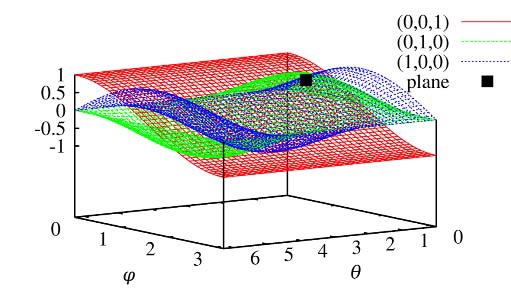
For the standard implementation of the 2D Hough transform, the Hough space is divided into $N_\rho\times N_\theta$ rectangular cells. The size of the cells is variable and is chosen problem-dependent. Using the same subdivision for the 3D Hough space by dividing it into cuboid cells results in the patches seen in Figure 3. The cells closer to the poles are smaller and comprise less normal vectors. This means voting favors the larger equatorial cells.

Accumulator Cube

We can also project the unit sphere $S^2$ onto the smallest cube that contains the sphere using the diffeomorphism:$$\begin{equation}\phi:S^2\to\mathrm{cube},s\mapsto\|s\|_\infty.\tag{3}\label{eq:3}\end{equation}$$

Each face of the cube is divided into a regular grid, which is shown in Figure 4. With this design of the accumulator, the difference of size between the patches on the unit sphere is negligible.

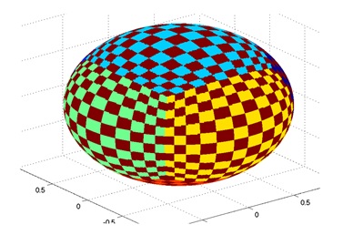
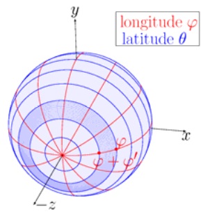
Accumulator Ball

The commonly used design, the accumulator array, which is shown in Figure 3, causes the irregularity between the patches on the unit sphere. To solve this issue, we can simply customize the resolution in polar coordinates depending on the position of the sphere. The resolution of the longitude $\phi$ is kept as for the accumulator array, which is defined as $\phi^\prime$. In the $\theta$ direction, the largest latitude circle is the equator located at $\phi=0$. For the unit sphere it has the $l_\text{max}=2\pi$. The length of the latitude circle in the middle of the segment located above $\phi_i$ is given by $l_i=2\pi(\phi+\phi^\prime)$. The step width in $\theta$ direction for each slice is now computed as $\theta_{\phi_i}=\frac{360^\circ\cdot l_\text{max}}{l_i\cdot N_\theta}$, where $N_\theta$ is a constant that can be customized. The resulting design is illustrated in Figure 5.