In geometry processing, Tutte embedding, also known as barycentric embedding, can be used for mesh parameterization by fixing the boundary vertices of the mesh on a certain convex polygon, and building a crossing-free straight-line embedding with the interior vertices inside the convex boundary.
Implementation of Tutte Embedding
In order to implement a Tutte embedding, we have to use two vectors $\mathbf{u}$ and $\mathbf{v}$ to store the parameterized coordinates, and another two vectors $\bar{\mathbf{u}}$ and $\bar{\mathbf{v}}$ to store the boundary vertices. For the interior vertex $i$, we can directly apply the following equation to it to build the barycentric mapping:$$\begin{equation}\sum_{}a_{i,j}\begin{pmatrix}u_j\\v_j\end{pmatrix}-a_{i,i}\begin{pmatrix}u_i\\v_i\end{pmatrix}=0,\tag{1}\label{eq:1}\end{equation}$$where $j$ denotes the adjacent vertices of $i$.
For those vertices on the boundary, we use the equation below and set $a_{i,i}=1$, to have them fixed on a convex shape:$$\begin{equation}\sum_{}a_{i,i}\begin{pmatrix}u_i\\v_i\end{pmatrix}=\begin{pmatrix}\bar{u}_i\\\bar{v}_i\end{pmatrix}.\tag{2}\label{eq:2}\end{equation}$$
Thus, we can build the two linear systems below:$$\begin{equation}\begin{cases}\mathbf{A}\mathbf{u}=\bar{\mathbf{u}},\\\mathbf{A}\mathbf{v}=\bar{\mathbf{v}},\end{cases}\tag{3}\label{eq:3}\end{equation}$$where $\mathbf{A}=(a_{i,j})$ is a sparse matrix storing all the weights $a_{i,j}$. And we can find the parameterized coordinates by solving for the two linear systems.
I chose a disk as the convex shape for fixing the boundary vertices and used the geometry-processing-js library for the data structure of meshes.
Weighting Schemes
I tried three different weight sets, namely the uniform Laplacian weights, the Laplace-Beltrami weights, and the mean value weights.
Uniform Laplacian Weights
The uniform Laplacian weight set is easiest to build, but it does not take the geometric feature of the mesh into consideration. We can simply set the entries of the weight matrix in the following manner:$$\begin{equation}\begin{cases}a_{i,j}=1,\\a_{i,i}=-\sum_{}a_{i,j}=-D_i,\end{cases}\tag{4}\label{eq:4}\end{equation}$$where $D_i$ is the degree of vertex $i$, i.e., the number of edges connecting $i$.
Laplace-Beltrami Weights
We can also derive weights from the Laplace-Beltrami operator:$$\begin{equation}\begin{cases}a_{i,j}=\frac{1}{2A_i}(\cot\alpha_{i,j}+\cot\beta_{i,j}),\\a_{i,i}=-\sum_{}a_{i,j},\end{cases}\tag{5}\label{eq:5}\end{equation}$$where $A_i$ denotes the area of the Voronoi region of the vertex $i$, $\alpha_{i,j}$ and $\beta_{i,j}$ denote respectively the two corners opposite to the edge $(i,j)$, as shown in Figure 1.
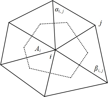
For calculating the value of $A_i$, we can use:$$\begin{equation}A_i=\frac{1}{8}\sum_{}(\cot\alpha_{i,j}+\cot\beta_{i,j})\|\mathbf{x}_i-\mathbf{x}_j\|^2,\tag{6}\label{eq:6}\end{equation}$$where $\|\mathbf{x}_i-\mathbf{x}_j\|$ is the length of edge $(i,j)$.
As far as one triangle from the one-ring neighborhood of a vertex is concerned, which is shown in Figure 2, the Voronoi region inside that triangle can be calculated as:$$\begin{equation}W=\frac{1}{8}\sum_{}(\|\mathbf{x}_i-\mathbf{x}_j\|^2\cot\alpha+\|\mathbf{x}_i-\mathbf{x}_j\|^2\cot\beta).\tag{7}\label{eq:7}\end{equation}$$
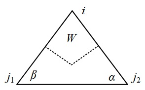
As the data structure of mesh is based on half-edge, we can simply find the neighbor of a certain half-edge by retrieving its previous half-edge, e.g., in Figure 2, half-edge $\langle j_2,i\rangle$ is previous to half-edge $\langle i,j_1\rangle$. Thus, by traversing outgoing half-edges associated on a vertex, we can easily calculate the Voronoi region of it using the following code snippet:
|
|
Mean Value Weights
The Laplace-Beltrami weight takes the geometry of a mesh into account, but it could be negative with obtuse triangles. Based on the mean value theorem, we can derive the mean value weights, which are always positive and generate one-to-one mappings:$$\begin{equation}\begin{cases}a_{i,j}=\frac{1}{\|\mathbf{x}_i-\mathbf{x}_j\|}(\tan\frac{\delta_{i,j}}{2}+\tan\frac{\gamma_{i,j}}{2}),\\a_{i,i}=-\sum_{}a_{i,j},\end{cases}\tag{8}\label{eq:8}\end{equation}$$where $\|\mathbf{x}_i-\mathbf{x}_j\|$ is the length of edge $(i,j)$, $\delta_{i,j}$ and $\gamma_{i,j}$ are two neighboring corners on both sides of edge $(i,j)$, as shown in Figure 3.
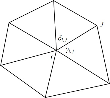
In the real implementation, like what we did in calculating the Voronoi region, we can still take advantage of the sequence of half-edges to find the corresponding corners:
|
|
Results and Conclusion
The results of Tutte embedding are shown in Figure 4, applied to different objects with different weight sets.
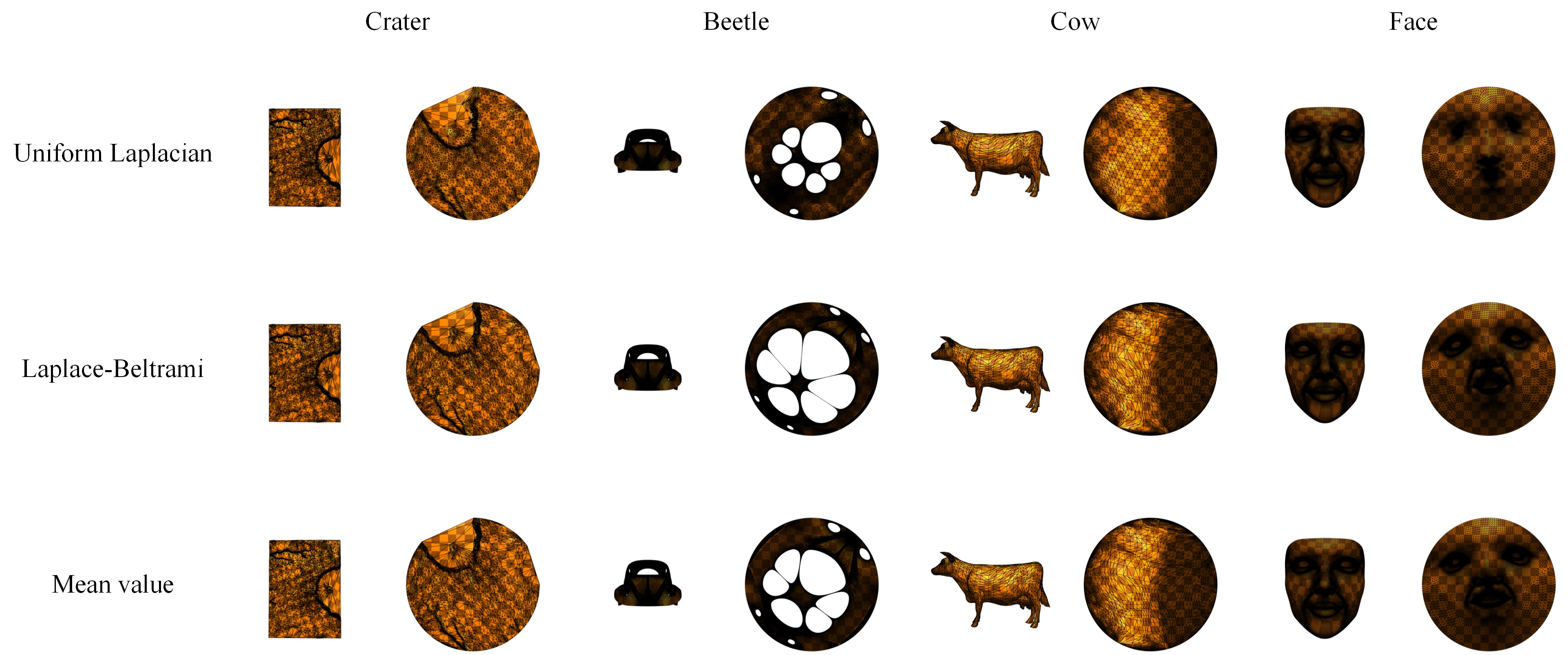
We can conclude from the results that the Laplace-Beltrami weight set and mean value weight set can better preserve the shape of triangles in the original mesh. This leads to the interior holes of a mesh to enlarge, which is clearly shown in the beetle. For better illustrating this property, we can take a close look at the mesh (Figure 5).
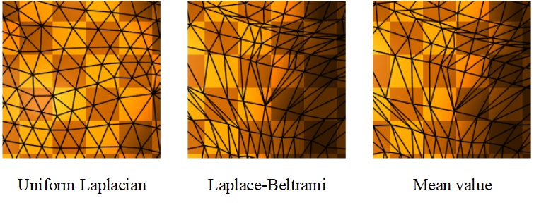
Figure 5 takes the same 200×200 pixels parts from the screenshots of the parametrizations of the cow object. It shows that the uniform Laplacian weight can cause the triangles on the parameterization to become more regular, but the triangles on the parameterized mesh of the Laplace-Beltrami weight and the mean value weight are more similar to those on the original mesh.
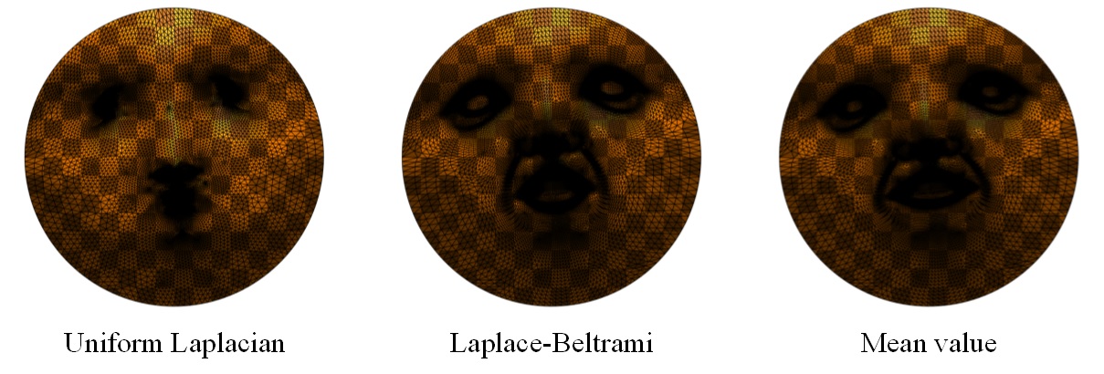
Besides, the Laplace-Beltrami weight and the mean value weight can even better preserve the patterns on the mesh. As shown in Figure 6, the features on the face object (i.e., the mouth and the eyes) are more distinguishable if we use the Laplace-Beltrami weight or the mean value weight.
I have also uploaded the project to this blog: /projects/tutte-embedding, we can go there to see how the algorithms work.